Algorithms used in the Reconstruction

In this section we describe the algorithms used in the reconstruction. Many of them make use of the concepts presented earlier. The order these algorithms are presented follows the actual process, from the 2D image in the beginning to the 3D model at the end.

Automatic phase

Preparing the image

Our goal is to acquire a set of lines from the image which will allow us to identify the correct vanishing points. The methodology described by Criminisi, does not make use of the color and lighting information of an image. To achieve detection of VPs we only need the structural information of the objects in the scene and more specifically the straight edges.

The first step is to perform a smoothing algorithm in the input image. Then we run an edge detector on the result. Our implementation uses a Gaussian smoothing algorithm and the Canny edge detector [1,10]. The edge detector is modified in order to break edges at points of high curvature. The result of this operation is a number of sets of pixels. Each set consists of pixels which form an almost straight line on the image.

Acquiring a set of lines

Methodology used in the SVR application.

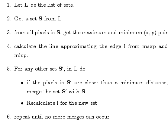
Some of the sets we obtained from the above process is possible to be parts of the same line. A merging algorithm is used to minimize the number of sets and is shown on table 1. The idea is that adjacent pixels are probably part of the same line.

**Table 1:** Algorithm for merging pixel sets that belong on the same line.
$\begin{table} \hrule \begin{enumerate} \item Let $\mathbf{L}$ be the list o... ... repeat until no more merges can occur. \end{enumerate} \hrule \end{table}$

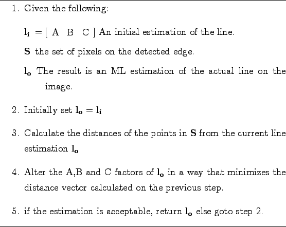
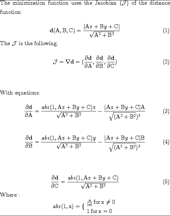
The final step is to calculate the best fitting line for each set of pixels. In order to achieve this we use a Maximum Likelihood estimation (MLE) technique based on the Levenberg-Marquardt algorithm [20]. The algorithm steps are shown on table 2. The minimization function used is shown on table 3.

**Table 2:** General steps of the ML estimation algorithm.
$\begin{table} \hrule \begin{enumerate} \item Given the following: \begin{d... ...eturn $\mathbf{l_o}$ else goto step 2. \end{enumerate} \hrule \end{table}$

**Table 3:** The minimization function of the MLE algorithm.
$\begin{table} \hrule The minimization function uses the Jacobian ($\cal{J}$) ... ...ox{for} \mathrm{x}=0 \end{array} \end{displaymath}\par \hrule \end{table}$

These types of algorithms are usually very time consuming. Fortunately in our case, we can start with a very good estimation. We use the first and the last pixel on the edge. These two points are probably very near the best line, due to the way the edge is traced in the previous steps. Given this, the MLE converges very fast.

Another approach.

The above combination of algorithms, were chosen over an alternative straight edge detection methodology, which was used in the early development stages of the SVR application.

This alternative method uses of a Hough transformation [21] after an unmodified Canny edge detector. The approach was abandoned for various reasons.

The hough transformation is a very CPU-intense algorithm, this means that when it is applied on a hight resolution image the completion of the edge detection stage could take unacceptably long time even on high end work stations.
Hough can be easily misled by artifacts in an image and detect existing lines. For example if an image contains a tree, the Canny result on the area of the tree leaves would be a cloud of pixels. This can easily trick hough, into producing false lines.
The threshold of hough has to be changed every time images of different resolution are processed in order to keep identifying the edges correctly. This means that heuristics had to be used to determine the best threshold, and in the worst cases, user interference was necessary⁵.

Tests with the hough version of the implementation and with the final MLE version, have shown that the later can be faster up to two or three orders-of-size depending on the input image.

Semi-automatic phase

Detecting the vanishing points.

The above steps can be completed automatically without any user input, except for some changes to the thresholds of the algorithms in order to achieve better results ⁶.

The next step in the reconstruction process is to identify the $\mathbf{VPs}$ from the intersections of the detected lines. In order to accomplish this step successfully, user guidance is necessary.

Various techniques [13,17] have been proposed in order to achieve an automated detection of the $\mathbf{VPs}$ . These methods provide ways of detecting more lines in the scene, based on patterns, and geometric structures. They do not try to distinguish between the lines that will lead to a correct result and to those which will not. The immediate consequence is that the `false lines' cause a high rate of false detections. This leaves the final selection of the correct $\mathbf{vp}$ from a set of candidates to the user.

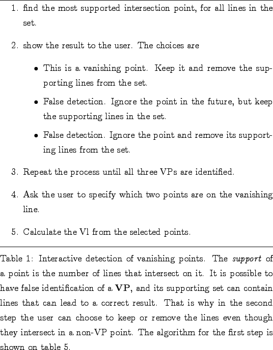
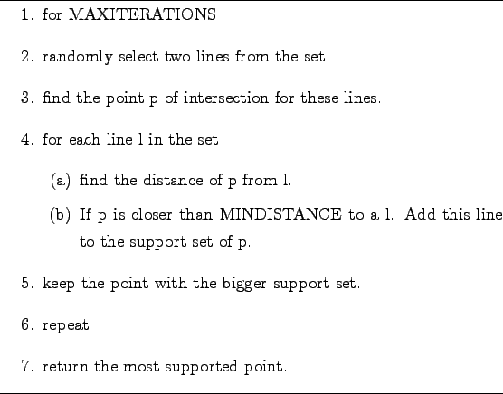
For this reason in our implementation a simple RANSAC like algorithm was chosen, over the proposed more complex techniques. The steps of the process are shown on table 4. The algorithm for choosing the most supported intersection point from all the intersections is shown on table 5.

$\begin{table} % latex2html id marker 397 \hrule \begin{enumerate} \item fin... ... The algorithm for the first step is shown on table \ref{t:alg4}.} \end{table}$

**Table 5:** Algorithm for choosing the best VP candidate.
$\begin{table} \hrule \begin{enumerate} \item for \textrm{MAXITERATIONS} \it... ... \item return the most supported point. \end{enumerate} \hrule \end{table}$

Computing the scale factors and camera position.

In section 3.2 we saw that we can compute the Homography matrix $\mathrm{H}$ with the equation 3. In order to completely define $\mathrm{H}$ we have to know some lengths on the scene. Also if we want to make measurements of heights (distances between horizontal planes and the ground) we must calculate the scale factor for the vertical direction.

We need the following information:

A reference height. A distance of a point in the image from the `ground'.
A reference length between two points on the `ground' plane.

Reference height

Given two points on the image, $\mathbf{x}$ and $\mathbf{x'}$ , and a reference length $\mathrm{Z_r}$ . Suppose that point $\mathbf{x}$ corresponds to a point on the ground in the scene, and $\mathbf{x'}$ corresponds to a point not on the ground in the scene such that the line $\mathbf{xx'}$ is vertical to the ground plane. We can compute the scale factor $\mathrm{A_z}$ directly from the equation:

$\begin{displaymath} \mathrm{A_z} =-\frac{\Vert \mathbf{x}\times\mathbf{x'}\Ver... ...bf{l}\cdot\mathbf{x})\Vert\mathbf{v_z}\times\mathbf{x'}\Vert} \end{displaymath}$

(10)

Reference Length

The exact analogue to the above equation can be used in order to calculate the $\mathrm{a}$ and $\mathrm{b}$ scale factors for the reference plane [5, p. 109].

Given a reference length on the ground, we calculate its two components on the coordinate system of $\mathbf{V_xOV_y}$ . $\mathbf{O}$ is the center of the world on the image with coordinates $\mathbf{O} = [\begin{array}{ccc} x_o & y_o & 0\end{array}]$ .

Let the two segments be:

$\mathrm{l_x}=[\begin{array}{cc} \mathrm{p_x} & \mathrm{{p_x}'}\end{array}]$ . The segment parallel to the $\mathbf{0V_y}$ axis. With length $\mathrm{X_r}$ .
$\mathrm{l_y}=[\begin{array}{cc} \mathrm{p_y} & \mathrm{{p_y}'}\end{array}]$ . The segment parallel to the $\mathbf{0V_x}$ axis. With length $\mathrm{Y_r}$ .

Then the equation 15 is transformed to :

$\begin{displaymath} \begin{array}{cc} \mathrm{a} =-\frac{\Vert \mathbf{p_x}\t... ... \mathbf{v_y} and \mathbf{v_z} \end{array} \end{array} \end{displaymath}$

(11)

and

$\begin{displaymath} \begin{array}{cc} \mathrm{b} =-\frac{\Vert \mathbf{p_y}\t... ... \mathbf{v_x} and \mathbf{v_z} \end{array} \end{array} \end{displaymath}$

(12)

With equations 16 and 17 we obtain the last two unknown scale factors $\mathrm{a}$ and $\mathrm{b}$ . Now we can compute any distance between objects on the ground plane as well as heights. The equations for these calculations where described on section 3.4.

At this point we have enough information to know the position of the camera. The coordinates are derived directly from the VPs as shown in eq. 18

$\displaystyle \mathrm{X_c}$	$\textstyle =$	$\displaystyle -det[\begin{array}{ccc} \mathrm{b}\mathbf{v}_y & \mathrm{A_z}\mathbf{v}_z & \mathbf{vl}\end{array}],$
$\displaystyle \mathrm{Y_c}$	$\textstyle =$	$\displaystyle det[\begin{array}{ccc} \mathrm{a}\mathbf{v}_x & \mathrm{A_z}\mathbf{v}_z & \mathbf{vl}\end{array}],$
$\displaystyle \mathrm{Z_c}$	$\textstyle =$	$\displaystyle -det[\begin{array}{ccc} \mathrm{a}\mathbf{v}_x & \mathrm{A_z}\mathbf{v}_y & \mathbf{vl}\end{array}],$	(13)
$\displaystyle \mathrm{W_c}$	$\textstyle =$	$\displaystyle det[\begin{array}{ccc} \mathrm{a}\mathbf{v}_x & \mathrm{A_z}\mathbf{v}_y & \mathbf{v}_z\end{array}]$

User guided reconstruction

With the techniques described this far, we can do the following two measurements:

height

Given two points in the image $\mathrm{p_1}$ and $\mathrm{p_2}$ , and given that:

If $\mathrm{P_1}$ and $\mathrm{P_2}$ are the points in the world for $\mathrm{p_1}$ and $\mathrm{p_2}$ respectively:

$\mathrm{P_1}$ is a point on the ground.

$\mathrm{P_1}$ is the image of $\mathrm{P_2}$ on the ground.

We can measure the distance $d(\mathrm{P_1},\mathrm{P_2})$ (using equation 6).

length

Given two points in the image $\mathrm{p_1}$ and $\mathrm{p_2}$ , and given that:

If $\mathrm{P_1}$ and $\mathrm{P_2}$ are the points in the world for $\mathrm{p_1}$ and $\mathrm{p_2}$ then both of them are on the ground plane.

We can measure the distance $d(\mathrm{P_1},\mathrm{P_2})$ (using equations 7 and 8).

The above are sufficient to recreate a scene with acceptable detail, if we have a method of identifying objects in the image. Various techniques are available for object segmentation and identification [5,3,9]. The basic structures that need to be defined before we can regain a 3D model are the following:

Lines vertical to the ground
Lines on the ground
Lines on planes vertical to the ground

Combinations of these objects can help us identify more complex ones. For example we can regain all three-dimensional information for a wall in a scene, if we know: (i) its two vertical lines ( $\mathrm{vl_1,vl_2}$ ) and (ii) a set of lines connecting the of-the-ground points of $\mathrm{vl_1}$ and $\mathrm{vl_2}$ (figure 3).

**Figure 3:** Reconstruction of a wall from the image. (a) The original image, the two red lines are the identified vertical lines. The blue lines are lines on the plane of the wall. (b) The reconstructed wall from a different perspective.
$\includegraphics[width=\textwidth height=!]{images/wallRec.eps}$

Automatic segmentation and object identification is beyond the scope of this work. In the next section, a user guided procedure is described, for identifying lines and planes in an image.

Footnotes

... necessary ⁵: Although the algorithm is no longer used in the procedure, the implementations where not removed from the project. This way comparing of the results is possible. Accessing these algorithms can be done through the svr application main window. The thresholds should first be changed to correspond to the needs of hough.
... results ⁶: This process can also be automated with suitable heuristics. For example when a high resolution image is used, the minimum edge threshold can be configured as a fraction of the image's diagonal.

jSVR

Single View Reconstruction